Friday, October 08, 2010

Foursquare outage post mortem

As many of you are aware, Foursquare had a significant outage this week. The outage was caused by capacity problems on one of the machines hosting the MongoDB database used for check-ins. This is an account of what happened, why it happened, how it can be prevented, and how 10gen is working to improve MongoDB in light of this outage.

It’s important to note that throughout this week, 10gen and Foursquare engineers have been working together very closely to resolve the issue.

Some history
Foursquare has been hosting check-ins on a MongoDB database for some time now. The database was originally running on a single EC2 instance with 66GB of RAM. About 2 months ago, in response to
increased capacity requirements, Foursquare migrated that single instance to a two-shard cluster. Now, each shard was running on its own 66GB instance, and both shards were also replicating to a slave for redundancy. This was an important migration because it allowed Foursquare to keep all of their check-in data in RAM, which is essential for maintaining acceptable performance.

The data had been split into 200 evenly distributed chunks based on user id. The first half went to one server, and the other half to the other. Each shard had about 33GB of data in RAM at this point, and the whole system ran smoothly for two months.

What we missed in the interim
Over these two months, check-ins were being written continually to each shard. Unfortunately, these check-ins did not grow evenly across chunks. It’s easy to imagine how this might happen: assuming certain subsets of users are more active than others, it’s conceivable that their updates might all go to the same shard. That’s what occurred in this case, resulting in one shard growing to 66GB and the other only to 50GB. [1]

What went wrong
On Monday morning, the data on one shard (we’ll call it shard0) finally grew to about 67GB, surpassing the 66GB of RAM on the hosting machine. Whenever data size grows beyond physical RAM, it becomes necessary to read and write to disk, which is orders of magnitude slower than reading and writing RAM. Thus, certain queries started to become very slow, and this caused a backlog that brought the site down.

We first attempted to fix the problem by adding a third shard. We brought the third shard up and started migrating chunks. Queries were now being distributed to all three shards, but shard0 continued to hit disk very heavily. When this failed to correct itself, we ultimately
discovered that the problem was due to data fragmentation on shard0. In essence, although we had moved 5% of the data from shard0 to the new third shard, the data files, in their fragmented state, still needed the same amount of RAM. This can be explained by the fact that Foursquare check-in documents are small (around 300 bytes each), so many of them can fit on a 4KB page. Removing 5% of these just made each page a little more sparse, rather than removing pages altogether.[2]

After the first day's outage it had become clear that chunk migration, sans compaction, was not going to solve the immediate problem. By the time the second day's outage occurred, we had already move 5% of the data off of shard0, so we decided to start an offline process to
compact the database using MongoDB’s repairDatabase() feature. This process took about 4 hours (partly due to the data size, and partly because of the slowness of EBS volumes at the time). At the end of the 4 hours, the RAM requirements for shard0 had in fact been reduced
by 5%, allowing us to bring the system back online.

Afterwards
Since repairing shard0 and adding a third shard, we’ve set up even more shards, and now the check-in data is evenly distributed and there is a good deal of extra capacity. Still, we had to address the fragmentation problem. We ran a repairDatabase() on the slaves, and
promoted the slaves to masters, further reducing the RAM needed on each shard to about 20GB.

How is this issue triggered?
Several conditions need to be met to trigger the issue that brought down Foursquare:
  • Systems are at or over capacity. How capacity is defined varies; in the case of Foursquare, all data needed to fit into RAM for acceptable performance. Other deployments may not have such strict RAM requirements.
  • Document size is less than 4k. Such documents, when moved, may be too small to free up pages and, thus, memory.
  • Shard key order and insertion order are different. This prevents data from being moved in contiguous chunks.

Most sharded deployments will not meet these criteria. Anyone whose documents are larger than 4KB will not suffer significant fragmentation because the pages that aren’t being used won’t be
cached.

Prevention
The main thing to remember here is that once you’re at max capacity, it’s difficult to add more capacity without some downtime when objects are small. However, if caught in advance, adding more shards on a live system can be done with no downtime.

For example, if we had notifications in place to alert us 12 hours earlier that we needed more capacity, we could have added a third shard, migrated data, and then compacted the slaves.

Another salient point: when you’re operating at or near capacity, realize that if things get slow at your hosting provider, you may find yourself all of a sudden effectively over capacity.

Final Thoughts
The 10gen tech team is working hard to correct the issues exposed by this outage. We will continue to work as hard as possible to ensure that everyone using MongoDB has the best possible experience. We are thankful for the support that we have received from Foursquare and our
community during this unfortunate episode. As always, please let us know if you have any questions or concerns.

[1] Chunks get split when they are 200MB into 2 100MB halves. This means that even if the number of chunks on each shard was the same, data size is not always so. This is something we are going to be addressing in MongoDB. We'll be making splitting balancing look for this imbalance so it can act upon it.

[2] The 10gen team is working on doing online incremental compaction of both data files and indexes. We know this has been a concern in non-sharded systems as well. More details about this will be coming in the next few weeks.


** copied from mongodb google group **

Friday, October 01, 2010

Database speed tests (mysql and postgresql) - part 3 - code

Here is the code structure

dbfuncs.php : is the file which contains classes and functions for firing queries on mysql and pgsql
mysqlinsert.php : creates and fires inserts on mysql
mysqlselect.php : creates and fires selects on mysql
pgsqlinsert.php : creates and fires inserts on pgsql
pgsqlselect.php : creates and fires selects on pgsql
benchmark.php : script used to control concurrency and number of queries per script

Please refer to http://jayant7k.blogspot.com/2010/09/database-speed-tests-mysql-and_29.html and http://jayant7k.blogspot.com/2010/09/database-speed-tests-mysql-and.html for benchmarks of selects and inserts respectively.

And the code....

dbfuncs.php
abstract class dbfuncs
{
  abstract function insertqry($qry);
  abstract function selectqry($qry);
  abstract function connectdb();

  public function log($str)
  {
    $file = "error.log";
    $fp = fopen($file, "a");
    fwrite($fp, "$str\n");
    fclose($fp);
  }
}

class mysqldb extends dbfuncs
{
  private $user = "root";
  private $pass = "jayant";
  private $host = "localhost";
  //private $port = 3307;
  private $socket = "/tmp/mysql.sock";
  private $database = "benchmark";

  public $db;

  function __construct()
  {
    $this->connectdb();
  }

  public function connectdb()
  {
    $this->db = mysql_connect($this->host.':'.$this->socket, $this->user, $this->pass) or die(mysql_error())
    mysql_select_db($this->database, $this->db);
  }

  public function insertqry($qry)
  {
    if(!mysql_ping($this->db))
      $this->connectdb();

    mysql_query($qry, $this->db) or $this->log(mysql_error());
  }

  public function selectqry($qry)
  {
    if(!mysql_ping($this->db))
      $this->connectdb();

    $rs = mysql_query($qry, $this->db) or $this->log(mysql_error());
    return $rs;
  }
}

class pgsqldb extends dbfuncs
{
  private $dns = "host=localhost port=5432 user=jayant password=12qwaszx dbname=benchmark";

  public $db;

  function __construct()
  {
    $this->connectdb();
  }

  public function connectdb()
  {
    $this->db = pg_connect($this->dns) or die(pg_last_error());
  }

  public function insertqry($qry)
  {
    if(!pg_ping($this->db))
      connectdb();

    pg_query($this->db, $qry) or $this->log(pg_last_error($this->db));
  }

  public function selectqry($qry)
  {
    if(!pg_ping($this->db))
      $this->connectdb();

    $rs = pg_query($this->db, $qry) or $this->log(pg_last_error($this->db));
    return $rs;
  }
}

function logtime($str)
{
    $file = "benchmark.log";
    $fp = fopen($file, "a");
    fputs($fp, $str);
    fclose($fp);
}

mysqlinsert.php
include "dbfuncs.php";

$scriptno = $argv[1]+1;
$count = $argv[2];

$mysql = new mysqldb();
$start = microtime(true);
for($x=0; $x<$count; $x++)
{
  $xx = $x*$scriptno;
  $qry = "insert into data (val, txt) values ('$xx','$x in $scriptno')";
  $mysql->insertqry($qry);
}
$end = microtime(true);
$log = "\nMysql innodb Time to insert $count in run $scriptno = ".($end-$start);
logtime($log);

pgsqlinsert.php
include "dbfuncs.php";

$scriptno = $argv[1]+1;
$count = $argv[2];

$mysql = new pgsqldb();
$start = microtime(true);
for($x=0; $x<$count; $x++)
{
  $xx = $x*$scriptno;
  $qry = "insert into data (val, txt) values ('$xx','$x in $scriptno')";
  $mysql->insertqry($qry);
}
$end = microtime(true);
$log = "\nAvg Pgsql Time to insert $count in run $scriptno = ".($end-$start);
logtime($log);

mysqlselect.php
include "dbfuncs.php";

$scriptno = $argv[1]+1;
$count = $argv[2];

$mysql = new mysqldb();
$start = microtime(true);
for($x=0; $x<$count; $x++)
{
  $xx = $x*$scriptno;
  $qry = "select * from `data` where val ='$xx'";
  $mysql->selectqry($qry);
}
$end = microtime(true);
$log = "\nMysql innodb Time to select $count in run $scriptno = ".($end-$start);
logtime($log);

pgsqlselect.php
include "dbfuncs.php";

$scriptno = $argv[1]+1;
$count = $argv[2];

$mysql = new pgsqldb();
$start = microtime(true);
for($x=0; $x<$count; $x++)
{
  $xx = $x*$scriptno;
  $qry = "select * from data where val ='$xx'";
  $mysql->selectqry($qry);
}
$end = microtime(true);
$log = "\nPgsql Time to select $count in run $scriptno = ".($end-$start);
logtime($log);

benchmark.php
$count = 100000;
$concurrency = 40;

for($i=0; $i<$concurrency; $i++)
{
   exec("php -q mysqlselect.php $i $count > /dev/null &");
//   exec("php -q pgsqlselect.php $i $count > /dev/null &");
//   exec("php -q mysqlinsert.php $i $count > /dev/null &");
//   exec("php -q pgsqlinsert.php $i $count > /dev/null &");
}

All test runs were individual - meaning that only one script was run at a time with different count and concurrency. For inserts $count was set to 10,000 and for selects $count was set to 100,000 while $concurrency kept on varying.

I am using ubuntu 10.04 with 32 bit kernel 2.6.32-24 and ext4 file system. And my system has around 3GB of RAM and Intel Core 2 DUO T5870 @ 2.0 GHz.

Wednesday, September 29, 2010

Database speed tests (mysql and postgresql) - part 2

Here is the comparison between mysql and postgresql for selects (only). I had used the same table that i had created earlier http://jayant7k.blogspot.com/2010/09/database-speed-tests-mysql-and.html while comparing insertion speed. I have created approximately 1,000,000 records in the table and ran selects on them. I also modified the configuration of both mysql and postgresql to enable faster selects.

Mysql

In mysql I specially disabled query_cache - the reason being that I would use innodb for tables with large number of inserts - due to its support for row level locking. And with every insert t
he query cache is marked as dirty. So enabling query cache would lead to caching of queries which will not be the scenario in a live setup.

Mysql Configuration :
innodb_buffer_pool_size = 256MB
key_buffer_size = 256MB
read_buffer_size = 512KB
sort_buffer_size = 512KB
query_cache_size = 0
thread_cache_size = 32
table_open_cache = 64

table information :
No of records : 9755366
data (idb) size : 692 MB

Mysql : (time for 100000 selects)

Avg time for 500000 selects with concurrency = 5 : 58.67
Avg time for 1000000 selects with concurrency = 10 : 122.8
Avg time for 2000000 selects with concurrency = 20 : 225.67
Avg time for 3000000 selects with concurrency = 30 : 351.66
Avg time for 4000000 selects with concurrency = 40 : 452.3


PostgreSQL :

Mysql has better table compression as compared to postgres. Same data in innodb is of around 700 MB while that in Postgres is of around 900 MB.

Postgres configuration :
shared_buffers = 128MB
work_mem = 1MB
random_page_cost = 4.0
effective_cache_size = 256MB


table information :
No of records : 9755366
data size : 912 MB

Pgsql : (time for 100000 selects)

Avg time for 500000 selects with concurrency = 5 : 86.8
Avg time for 1000000 selects with concurrency = 10 : 144.74
Avg time for 2000000 selects with concurrency = 20 : 274.37
Avg time for 3000000 selects with concurrency = 30 : 402.92
Avg time for 4000000 selects with concurrency = 40 : 528.17


Mysql seems to perform better with selects. The graph also shows that with increase in concurrency, selects in innodb take lesser time than that in postgresql.

So, why would you switch from mysql to postgresql - only if you have a very high ratio of inserts as compared to selects. The benefit in inserts outweigh the loss in selects to some extent.

Monday, September 27, 2010

Database speed tests (mysql and postgresql) - part 1

There has been major changes in mysql and postgres over a couple of years. Mysql has been focusing on improving and optimizing innodb. Postgres on the other hand has been focusing on database replication and hot standby.

Recently postgres came out with version 9.0 which has built-in replication and hot standby - the two most requested feature in postgresql. Earlier people used to shy away from postgres because there was no proper "easily deployable" solution available for replication. Now with this release, postgres had taken a major step forward. Here http://www.postgresql.org/docs/9.0/static/release-9-0 is a list of features that has been introduced in postgres 9.0

Mysql has released the rc version of Mysql 5.5 which has a bunch of improvements over the previous version of mysql. Support for multi-core cpus, Changes in Innodb for effective use of available I/O capacity, semisynchronous replication - are some of the features that mysql 5.5 promices. Here is a list of all the new features in MySQL 5.5 http://dev.mysql.com/doc/refman/5.5/en/mysql-nutshell.html

It has been a long time, since posted my last benchmark http://jayant7k.blogspot.com/2008/06/mysql-versus-postgresql.html. And i believe it is time i do some rough benchmarks and post it out. The scope is to check out innodb tables in mysql 5.5.6 versus the tables in postgresql 9.0. I am focusing only on inserts and selects. And i will be benchmarking pure inserts and selects only. Thie blog focuses only on inserts. I will be focusing on selects in my next blog. I am running these tests on my laptop which has a Intel Core 2 Duo T5870 @ 2.00 GHz and 3 GB of RAM

I have created a simple php script to perform the benchmark. Which spawns out multiple php scripts that work on background. Let me know if you need the scripts and i will share it with you.

Mysql:

Innodb Settings in my.cnf :

innodb_buffer_pool_size = 256M
innodb_additional_mem_pool_size = 8M
innodb_log_file_size = 64M
innodb_log_buffer_size = 8M
innodb_flush_log_at_trx_commit = 1
innodb_lock_wait_timeout = 50
innodb_file_per_table

Table structure :
CREATE TABLE `data` (
`id` int(11) NOT NULL AUTO_INCREMENT,
`val` int(11) NOT NULL,
`txt` varchar(20) DEFAULT NULL,
PRIMARY KEY (`id`),
KEY `idx_val` (`val`)
) ENGINE=InnoDB DEFAULT CHARSET=latin1


Avg Time for 20000 inserts with concurrency of 2 : 1367 seconds
Load on machine : 3.4
size on disk : 9 MB

Avg Time for 50000 inserts with concurrency of 5 : 1537.2 seconds
Load on machine : 4.6
Size on disk : 13 MB

Avg Time for 100000 inserts with concurrency of 10 : 1255
Load on machine : 3.5
Size on disk : 17 MB

Avg Time for 200000 inserts with concurrency of 20 : 1403
Load on machine : 4.2
Size on disk : 26 MB

Time for 400000 inserts with concurrency of 40 : 1730
Load in machine : 6.6
Size on disk : 52 MB


Postgresql :

Settings in postgresql.conf:
shared_buffers = 64MB
work_mem = 1MB
synchronous_commit = on


Table structure :
Column | Type | Modifiers | Storage | Description
--------+-----------------------+---------------------------------------------------+----------+-------------
id | integer | not null default nextval('data_id_seq'::regclass) | plain |
val | integer | not null | plain |
txt | character varying(20) | | extended |
Indexes:
"data_pkey" PRIMARY KEY, btree (id)
"idx_val" btree (val)
Has OIDs: no

Avg Time for 20000 inserts with concurrency of 2 : 221.3 seconds
Load on machine : 2.0
size on disk : 2 MB

Avg Time for 50000 inserts with concurrency of 5 : 232 seconds
Load on machine : 2.0
Size on disk : 4.8 MB

Avg Time for 100000 inserts with concurrency of 10 : 248.75 seconds
Load on machine : 4.0
Size on disk : 9.8 MB

Avg Time for 200000 inserts with concurrency of 20 : 276.34
Load on machine : 3.6
Size on disk : 19 MB

Time for 400000 inserts with concurrency of 40 : 350.11
Load in machine : 5.8
size on disk : 38 MB


The graph shows that mysql is heavy as compared to pgsql. The base timings are almost 5 times more in mysql as compared to pgsql. Also as the concurrency goes up the time required for inserts in mysql spikes up more steeply as compared to that required for postgres.

I did a sample run on mysql by turning innodb_flush_logs_at_trx_commit=2 and the benefit I got was a lot

Avg Time for 20000 inserts with concurrency of 2 (innodb_flush_logs_at_trx_commit=2) : 5.2 seconds
Avg Time for 100000 inserts with concurrency of 10 (innodb_flush_logs_at_trx_commit=2) : 18.69 seconds

Similarly i disabled synchronous_commit on postgres and did a sample run

Avg Time for 20000 inserts with concurrency of 2 (synchronous_commit = off) : 2.95 seconds
Avg Time for 100000 inserts with concurrency of 10 (synchronous_commit = off) : 15.06 seconds

PS : The average time is the time for 10000 inserts (inserts per instance)

Lets see what do the selects tell - in the next blog.

Tuesday, September 14, 2010

Strategies to address scalability

There are some very fundamental scalability strategies which i will try to list here. These may have detailed and varied implementations.

  • Horizontal scalability - distribute the load : A very basic strategy for scalability is the ability to distribute the load or the requests across multiple processing units. Your code should be modular enough to allow horizontal scalability. Also the less information is shared among multiple requests, the easier it would be for you to scale horizontally. You should aim for a shared-nothing architecture
  • Sharding or partitioning is another way of scaling horizontally. The main idea here is to spread the load across many components by routing an individual request to a component that owns the data specific to that request. So you divide the complete data across multiple components and spread the requests among the components. There are two ways of creating shards:

    • Vertical partitioning : Spread the load across multiple processing units by distributing the functionalities across the components. So separate functions are being handled by different processing units. Column based databases are a very good example of vertical partitioning.
    • Horizontal Partitioning : Spread a single type of data element across multiple processing units. It is also referred to as hashing. Hashing based on userid to spread users across multiple datapoints can be an example of horizontal partitioning.
  • Parallelization is another way of achieving scalability. Parallelization can be achieved by working on the same task in parallel on multiple processing units. For example a web page having
    multiple components can process and fetch the components in parallel from multiple processing units.
  • Queueing or batch processing : Queueing and processing data in batches also provide a solution to scalability. Because the overhead of an operation is ammortized across multiple requests.< /li>
  • Relaxation of data constraints : Many different techniques and trade-offs with regards to how fast data can be accessed/processed or stored fall in this strategy. Caching, giving away fore
    ign keys and replication or denormalization of data are some of the examples of this strategy.

Ofcourse scalability cannot be addressed using only one of these strategies. The solution for scalability would depend on how the data is held and what compromises are we able to make with it. The solution might be a combination of a few of these strategies and more.

Original post : http://thebigsoftwareblog.blogspot.com/2010/08/scalability-fundamentals-and.html

Friday, September 10, 2010

Converting myisam tables to innodb

Why should you convert myisam tables to innodb ?

For the perfectly simple reason that innodb tables do not get locked by concurrent selects & inserts. So if you find that your myisam table is suffering for too many locks - due to concurrent selects and inserts, it is time for you to covert the table to innodb.

The simple query which does the trick is

Alter table myisam_table_name engine = innodb;

This query is good for small tables, which get converted in a flash (I am refering to tables smaller than 1 GB). But when you try to run this query to alter bigger tables, it takes a huge amount of time. You have to wait - maybe hours if not days to get your job done.

Recently I had a 30 GB table which i wanted to convert to innodb and the alter query went on for 3 days after which i gave up and killed the query. And then went on finding ways to make this alter happen fast.

There are multiple ways to make your alter fast -

1. create a temporary table with engine = innodb, disable unique checks and insert into the table in batches. The sequence of sql statements for this are

create table new_table_name like old_table_name;
alter table new_table_name engine = innodb;
set unique_checks=0;
// loop till all records are ported
insert into new_table_name select * from old_table_name where key > something and key <= something; set unique_checks=1;

If you have UNIQUE constraints on secondary keys, this speeds up a table import by turning off the uniqueness checks temporarily during the import operation.

2. Increase the buffers. In order to achieve higher I/O, you can increase the buffers - innodb_buffer_pool and innodb_log_file_size. If you are using a 64 bit machine - make the innodb_buffer_pool almost 50% of your available memory and innodb_log_file_size to around 128 MB (atleast) - you can make it 256MB to be a little more aggressive and 512 MB to be very aggressive. But it should be less than 25% of your innodb_buffer_pool size.

in my.cnf enter

innodb_buffer_pool = 2048M
innodb_log_file_size = 256M
innodb_log_buffer_size = 16M


Stop mysql.
Delete the ib_logfile0 & ib_logfile1.
start mysql.

Now running the alter query should be much faster.

A combination of both the above methods could be even more beneficial. Remember to re-tune your innodb settings - as per your requirement before putting live load on the server.

BTW, i tried using the second method to alter the 30 GB table, and looking at its speed, it seems that it will be done in around 10 hours - instead of the 3 days it took earlier.

Tuesday, September 07, 2010

Hashing algos : Consistent Hashing

Hashing is a way of mapping keys to locations. Normally you would hash by using a simple Key%n algorithm - which ensures that keys are mapped evenly across n splits. The problem with this algo is that adding or removing a node (or a split) would require a complete rehash of all the keys. And if you have a huge data set, it is ideally not feasable to rehash and re-distribute the keys.

Consistent hashing is a way of hashing that ensures that adding or removing a slot or node does not change the mapping of keys to slots significantly. When using consistent hashing, only K/n keys need to be remapped on average - where K is the number of keys and n is the number of slots.

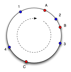
The way this works is that both keys and slots are mapped to edges of a circle. Meaning that all slots are mapped on to a series of angles around a circle. And the bucket where each item should be stored is chosen by selecting the next highest angle which an available bucket maps to. So, each bucket contains resources mapping to an angle between it and the next smallest angle. If a bucket becomes unavailable, the keys being mapped to that bucket get mapped to the next highest bucket (or the next bucket in the circle). So, only keys which were in the bucket which became unavailable is lost. Similarly when a bucket is added, the keys between the new bucket and the next smallest bucket is mapped to the new bucket. Keys which should be associated with the new bucket and were stored previously will become unavailable.

figure 2
figure 1

Here is an example. Objects 1,2,3 and 4 map to slots A,B and C. To find which slot an object goes in, we move around the circle until we find a slot. So here objects 1 and 4 go into slot A, 2 goes into slot B and 3 goes into slot C. If C is removed, object 3 would belong to slot A. If another slot D is added as shown in figure 2, it will take objects 3 and 4 and only leave object 1 belonging to A.

Lets look at a php example which does consistent hasing us.
<?php
class ConsistentHasher
{
  private $nodeDistribution;
  private $virtualNodes;

  // nodeDistribution is the replica count per node.
  public function __construct($nodenames, $nodedistribution)
  {
    $this->nodeDistribution = $nodedistribution;
    $this->virtualNodes = array();

    for($i=0; $i<count($nodenames); $i++)
    {
      $this->addNode($nodenames[$i]);
    }
  }

  // The addNode() function takes a name and creates virtual nodes (or replicas) by 
  // appending the index of the local loop to the node name.
  // The hash value of a virtual node is an MD5 hash, base converted into an integer. 
  // The virtual node is added to a list and sorted by its value so that we ensure 
  // a lowest to highest traversal order for looking up previous and next virtual nodes
  public function addNode($name)
  {
    for($i=0; $i<$this->nodeDistribution; $i++)
    {
      //int representation of $key (8 hex chars = 4 bytes = 32 bit)
      $virtualNodeHashCode = base_convert(substr(md5($name.$i, false),0,8),16,10);
      $this->virtualNodes[$name.$i] = $virtualNodeHashCode;
    }
    asort($this->virtualNodes, SORT_NUMERIC);
  }

  public function dump()
  {
    print_r($this->virtualNodes);
    echo "\n\n";
  }

  public function sortCompare($a, $b)
  {
    if($a == $b)
    {
      return 0;
    }
    return ($a < $b) ? -1 : 1;
  }

  // The removeNode() function takes a name and removes its corresponding virtual nodes 
  // from the virtualNode list.
  // We then resort the list to ensure a lowest to highest traversal order.
  public function removeNode($name)
  {
    for($i=0; $i<$this->nodeDistribution; $i++)
    {
      unset($this->virtualNodes[$name.$i]);
    }
    asort($this->virtualNodes, SORT_NUMERIC);
  }

  // The hashToNode() function takes a key and locates the node where its value resides.
  // We loop through our virtual nodes, stopping before the first one that has a
  // hash greater than that of the key’s hash.
  // If we come to the end of the virtual node list, we loop back to the beginning to 
  // form the conceptual circle.

  public function hashToNode($key)
  {
    $keyHashCode = base_convert(substr(md5($key, false),0,8),16,10);
    $virtualNodeNames = array_keys($this->virtualNodes);
    $firstNodeName = $virtualNodeNames[0];
    $lastNodeName = $virtualNodeNames[count($virtualNodeNames)-1];
    $prevNodeName = $lastNodeName;

    foreach($this->virtualNodes as $name => $hashCode)
    {
      if($keyHashCode < $hashCode)
        return $prevNodeName;

      if($name == $lastNodeName)
        return $firstNodeName;

      $prevNodeName = $name;
    }
    return $prevNodeName;
  }
}

// demo

$hash = new ConsistentHasher(array("node1","node2","node3","node4","node5"),10);
$hash->dump();

$hash->removeNode("node2");
$hash->dump();

$hash->addNode("node6");
$hash->dump();

echo $hash->hashToNode("testing123")."\n";
echo $hash->hashToNode("key1111")."\n";
echo $hash->hashToNode("data4444")."\n";
?>


Here is a library which provides consistent hasing for php
http://code.google.com/p/flexihash/

Memcache is a widely used distributed cache which uses consistent hashing very efficiently to map keys to caching nodes.

References:
http://en.wikipedia.org/wiki/Consistent_hashing
http://www.osconvo.com/post/view/2010/9/1/distributed-hashing-algorithms-by-example-consistent-hashing

Monday, August 23, 2010

Troubleshooting : mysql server has gone away

When running query against a database the following error can be generated:

ERROR 2006 (HY000) at line NNN: MySQL server has gone away

Where "NNN" is the line number of the script currently being run where the error occurred.

Possible Causes and Resolution

This is a general error which can have a number of possible causes. The one certainty is that the MySQL database is no longer listening on the connection - but this does not necessarily mean that MySQL is no longer available.

Possible causes:

MySQL has crashed.
Check that MySQL is still running on the server. If it is not running and this was not a planned shutdown then it is reasonable to conclude that MySQL has crashed. I personally have never experienced this, but if it happens then investigate whether you can upgrade to a newer version.

MySQL has been shutdown.
Check that MySQL is still running, if it is not and it was shut down (accidentally or intentionally) then that is the cause of the problem. Restart MySQL.

Network connectivity has failed.
Even if the database is still up, is it possible to contact the server? If you can ping the server (or MySQL is running no the localhost) then basic network connectivity is not the problem.

MySQL networking has failed
The problem may be the MySQL connection. If the query was trying to transfer a large block of data then the MySQL packet-size may be set too small.

Try increasing the value of max_allowed_packet and restart the MySQL database service. In MySQL Administrator select "Startup Variables" andon the "Advanced Networking" tab thsi is shown under "Data / Memory size" and is labeled as "Max. packet size." The default is 1MB and one of my systems now runs at 16MB.

The database connection has timed out and thus the SQL has failed.
Try increasing the wait_timeout, or reconnecting just before firing the query.

Modified after copying from http://www.cryer.co.uk/brian/mysql/trouble_mysql_gone_away.htm

Thursday, August 05, 2010

Linked-in data infrastructure

Jay Kreps of LinkedIn presented some informative details of how they process data at the recent Hadoop Summit. Kreps described how LinkedIn crunches 120 billion relationships per day and blends large scale data computation with high volume, low latency site serving.

Much of LinkedIn's important data is offline - it moves fairly slowly. So they use daily batch processing with Hadoop as an important part of their calculations. For example, they pre-compute data for their "People You May Know" product this way, scoring 120 billion relationships per day in a mapreduce pipeline of 82 Hadoop jobs that requires 16 TB of intermediate data. This job uses a statistical model to predict the probability of two people knowing each other. Interestingly they use bloom filters to speed up large joins, yielding a 10x performance improvement.

They have two engineers who work on this pipeline, and are able to test five new algorithms per week. To achieve this rate of change, they rely on A/B testing to compare new approach to old approaches, using a "fly by instruments" approach to optimize results. To achieve performance improvements, they also need to operate on large scale data - they rely on large scale cluster processing. To achieve that they moved from custom graph processing code to Hadoop mapreduce code - this required some thoughtful design since many graph algorithms don't translate into mapreduce in a straightforward manner.

LinkedIn invests heavily in open source,with the goal of building on best in class components, recruiting community involvement. Two of these open source projects were presented as central to their data infrastructure. Azkaban is an open source workflow system for Hadoop, providing cron-like scheduling and make-like dependency analysis, including restart. It is used to control ETL jobs that push database and event logs to their edge server storage, Voldemort.

Voldemort is LinkedIn's NoSQL key/value storage engine. Every day they push out an updated multi-billion edge probabilistic relationship graph to their live site for querying in rendering web pages.  This data is read-only: it is computed in these cluster jobs, but then filtered through a faceted search in realtime, e.g., restricting to certain companies of interest, or excluding people the user has indicated are not known to them. It grew out of their problems using databases to solve this problem, which required sharding and devolved into a system with a fulltime manual job moving data around.  Voldemort is fully distributed and decentralized, and supports partitioning and fail over.

LinkedIn updates their live servers with a large scale parallel fetch of results from Hadoop into Voldemort, warms up the cache, then institutes an atomic switchover to the new day's data on each server separately. They keep the previous day's data in the server to allow near instantaneous fallback in case of problems with new data sets. LinkedIn builds an index structure in their Hadoop pipeline - this produces a multi-TB lookup structure that uses perfect hashing (requiring only 2.5 bits per key). This process trades off cluster computing resources for faster server responses; it takes LinkedIn about 90 minutes to build a 900 GB data store on a 45 node development cluster. They use Hadoop to process massive batch workloads, taking their Hadoop cluster down for upgrades periodically, whereas their Voldemort servers never go down.

For more details, see the slides from the presentation.

Copied from http://www.infoq.com/news/2010/08/linkedin-data-infrastructure

Thursday, July 29, 2010

Cassandra Data model : WTF is a supercolumn

BTW: this is long. If you’d rather have a PDF version of this you can download it here.

The Pieces

Let’s first go thru the building blocks before we see how they can all be stuck together:

Column

The column is the lowest/smallest increment of data. It’s a tuple (triplet) that contains a name, a value and a timestamp.

Here’s a column represented in JSON-ish notation:
{  // this is a column
    name: "emailAddress",
    value: "arin@example.com",
    timestamp: 123456789
}
That’s all it is. For simplicity sake let’s ignore the timestamp. Just think of it as a name/value pair.

Also, it’s worth noting is that the name and value are both binary (technically byte[]) and can be of any length.

SuperColumn

A SuperColumn is a tuple w/ a binary name & a value which is a map containing an unbounded number of Columns – keyed by the Column’s name. Keeping with the JSON-ish notation we get:
{   // this is a SuperColumn
    name: "homeAddress",
    // with an infinite list of Columns
    value: {
        // note the keys is the name of the Column
        street: {name: "street", value: "1234 x street", timestamp: 123456789},
        city: {name: "city", value: "san francisco", timestamp: 123456789},
        zip: {name: "zip", value: "94107", timestamp: 123456789},
    }
}
Column vs SuperColumn

Columns and SuperColumns are both a tuples w/ a name & value. The key difference is that a standard Column’s value is a “string” and in a SuperColumn the value is a Map of Columns. That’s the main difference… their values contain different types of data. Another minor difference is that SuperColumn’s don’t have a timestamp component to them.

Before We Get Rolling

Before I move on I wanna simplify our notation a couple ways: 1) ditch the timestamps from Columns & 2) pull the Columns’ & SuperColumns’ names component out so that it looks like a key/value pair. So we’re gonna go from:
{ // this is a super column
    name: "homeAddress",
    // with an infinite list of columns
    value: {
        street: {name: "street", value: "1234 x street", timestamp: 123456789},
        city: {name: "city", value: "san francisco", timestamp: 123456789},
        zip: {name: "zip", value: "94107", timestamp: 123456789},
    }
}
to

 homeAddress: {
    street: "1234 x street",
    city: "san francisco",
    zip: "94107",
}
Grouping ‘Em

There’s a single structure used to group both the Columns and SuperColumns…this structure is called a ColumnFamily and comes in 2 varieties Standard & Super.

ColumnFamily

A ColumnFamily is a structure that contains an infinite number of Rows. Huh, did you say Rows? Ya – rows To make it sit easier in your head just think of it as a table in an RDBMS.

OK – each Row has a client supplied (that means you) key & contains a map of Columns. Again, the keys in the map are the names of the Columns and the values are the Columns themselves:
UserProfile = { // this is a ColumnFamily
    phatduckk: {   // this is the key to this Row inside the CF
        // now we have an infinite # of columns in this row
        username: "phatduckk",
        email: "phatduckk@example.com",
        phone: "(900) 976-6666"
    }, // end row
    ieure: {   // this is the key to another row in the CF
        // now we have another infinite # of columns in this row
        username: "ieure",
        email: "ieure@example.com",
        phone: "(888) 555-1212"
        age: "66",
        gender: "undecided"
    },
}
Remember: for simplicity we're only showing the value of the Column but in reality the values in the
map are the entire Column.
You can think of it as a HashMap/dictionary or associative array. If you start thinking that way then you’re are the right track.

One thing I want to point out is that there’s no schema enforced at this level. The Rows do not have a predefined list of Columns that they contain. In our example above you see that the row with the key “ieure” has Columns with names “age” and “gender” whereas the row identified by the key “phatduckk” doesn’t. It’s 100% flexible: one Row may have 1,989 Columns whereas the other has 2. One Row may have a Column called “foo” whereas none of the rest do. This is the schemaless aspect of Cassandra.

A ColumnFamily Can Be Super Too

Now, a ColumnFamily can be of type Standard or Super.

What we just went over was an example of the Standard type. What makes it Standard is the fact that all the Rows contains a map of normal (aka not-Super) Columns… there’s no SuperColumns scattered about.

When a ColumnFamily is of type Super we have the opposite: each Row contains a map of SuperColumns. The map is keyed with the name of each SuperColumn and the value is the SuperColumn itself. And, just to be clear, since this ColumnFamily is of type Super, there are no Standard ColumnFamily’s in there. Here’s an example:
AddressBook = { // this is a ColumnFamily of type Super
    phatduckk: {    // this is the key to this row inside the Super CF
        // the key here is the name of the owner of the address book

        // now we have an infinite # of super columns in this row
        // the keys inside the row are the names for the SuperColumns
        // each of these SuperColumns is an address book entry
        friend1: {street: "8th street", zip: "90210", city: "Beverley Hills", state: "CA"},

        // this is the address book entry for John in phatduckk's address book
        John: {street: "Howard street", zip: "94404", city: "FC", state: "CA"},
        Kim: {street: "X street", zip: "87876", city: "Balls", state: "VA"},
        Tod: {street: "Jerry street", zip: "54556", city: "Cartoon", state: "CO"},
        Bob: {street: "Q Blvd", zip: "24252", city: "Nowhere", state: "MN"},
        ...
        // we can have an infinite # of ScuperColumns (aka address book entries)
    }, // end row
    ieure: {     // this is the key to another row in the Super CF
        // all the address book entries for ieure
        joey: {street: "A ave", zip: "55485", city: "Hell", state: "NV"},
        William: {street: "Armpit Dr", zip: "93301", city: "Bakersfield", state: "CA"},
    },
}
Keyspace

A Keyspace is the outer most grouping of your data. All your ColumnFamily’s go inside a Keyspace. Your Keyspace will probably named after your application.

Now, a Keyspace can have multiple ColumnFamily’s but that doesn’t mean there’s an imposed relationship between them. For example: they’re not like tables in MySQL… you can’t join them. Also, just because ColumnFamily_1 has a Row with key “phatduckk” that doesn’t mean ColumnFamily_2 has one too.

Sorting

OK – we’ve gone through what the various data containers are about but another key component of the data model is how the data is sorted. Cassandra is not queryable like SQL – you do not specify how you want the data sorted when you’re fetching it (among other differences). The data is sorted as soon as you put it into the cluster and it always remains sorted! This is a tremendous performance boost for reads but in exchange for that benefit you’re going to have to make sure to plan your data model in a such a way that you’re able satisfy your access patterns.

Columns are always sorted within their Row by the Column’s name. This is important so i’ll say it again: Columns are always sorted by their name! How the names are compared depends on the ColumnFamilys CompareWith option. Out of the box you have the following options: BytesType, UTF8Type, LexicalUUIDType, TimeUUIDType, AsciiType, and LongType. Each of these options treats the Columns’ name as a different data type giving you quite a bit of felxibility. For example: Using LongType will treat your Columns’ names as a 64bit Longs. Let’s try and clear this up by taking a look at some data before and after it’s sorted:

// Here's a view of all the Columns from a particular Row in random order
    // Cassandra would "never" store data in random order. This is just an example
    // Also, ignore the values - they don't matter for sorting at all
    {name: 123, value: "hello there"},
    {name: 832416, value: "kjjkbcjkcbbd"},
    {name: 3, value: "101010101010"},
    {name: 976, value: "kjjkbcjkcbbd"}
So, given the fact that we’re using the LongType option, these Columns will look like this when they’re sorted:


    <!--
    ColumnFamily definition from storage-conf.xml
    -->
    <ColumnFamily CompareWith="LongType" Name="CF_NAME_HERE"/>

    // See, each Column's name is treated as a 64bit long
    // in effect, numerically ordering our Columns' by name
    {name: 3, value: "101010101010"},
    {name: 123, value: "hello there"},
    {name: 976, value: "kjjkbcjkcbbd"},
    {name: 832416, value: "kjjkbcjkcbbd"}
As you can see the Columns’ names were compared as if they were 64bit Longs (aka: numbers that can get pretty big). Now, if we’d used another CompareWith option we’d end up with a different result. If we’d set CompareWith to UTF8Type our sorted Columns’ names would be treated as a UTF8 encoded strings yielding a sort order like this:

<!--
    ColumnFamily definition from storage-conf.xml
    -->
    <ColumnFamily CompareWith="UTF8Type" Name="CF_NAME_HERE"/>

    // Each Column name is treated as a UTF8 string
    {name: 123, value: "hello there"},
    {name: 3, value: "101010101010"},
    {name: 832416, value: "kjjkbcjkcbbd"},
    {name: 976, value: "kjjkbcjkcbbd"}
The result is completely different!

This sorting principle applies to SuperColumns as well but we get an extra dimension to deal with: not only do we determine how the SuperColumns are sorted in a Row but we also determine how the Columns within each SuperColumn are sorted. The sort of the Columns within each SuperColumn is determined by the value of CompareSubcolumnsWith. Here’s an example:

// Here's a view of a Row that has 2 SuperColumns in it.
    // currently they're in some random order

    { // first SuperColumn from a Row
        name: "workAddress",
        // and the columns within it
        value: {
            street: {name: "street", value: "1234 x street"},
            city: {name: "city", value: "san francisco"},
            zip: {name: "zip", value: "94107"}
        }
    },
    { // another SuperColumn from same Row
        name: "homeAddress",
        // and the columns within it
        value: {
            street: {name: "street", value: "1234 x street"},
            city: {name: "city", value: "san francisco"},
            zip: {name: "zip", value: "94107"}
        }
    }
Now if we decided to set both CompareSubcolumnsWith & CompareWith to UTF8Type we’d have the following end result:

// Now they're sorted

    {
        // this one's first b/c when treated as UTF8 strings
        { // another SuperColumn from same Row

            // This Row comes first b/c "homeAddress" is before "workAddress"
            name: "homeAddress",

            // the columns within this SC are also sorted by their names too
            value: {
                // see, these are sorted by Column name too
                city: {name: "city", value: "san francisco"},
                street: {name: "street", value: "1234 x street"},
                zip: {name: "zip", value: "94107"}
            }
        },
        name: "workAddress",
        value: {
            // the columns within this SC are also sorted by their names too
            city: {name: "city", value: "san francisco"},
            street: {name: "street", value: "1234 x street"},
            zip: {name: "zip", value: "94107"}
        }
    }
I want to note that in the last example CompareSubcolumnsWith & CompareWith were set to UTF8Type but this doesn’t have to be the case. You can mix and match the values of CompareSubcolumnsWith & CompareWith as necessary.

The last bit about sorting I want to mention is that you can write a custom class to perform the sorting. The sorting mechanism is pluggable… you can set CompareSubcolumnsWith and/or CompareWith to any fully-qualified class name as long as that class implements org.apache.cassandra.db.marshal.IType (aka you can write custom comparators).

Example Schema

Alrighty – Now we’ve got all the pieces of the puzzle so let’s finally put ‘em all together and model a simple blog application. We’re going to model a simple app with the following specs:

support a single blog
we can have multiple authors
entries contain title, body, slug & publish date
entries can be associated with any # of tags
people can leave comments but cant register: they enter profile info each time (just keeping it simple)
comments have text, time submitted, commenter’s name & commenter’s name
must be able to show all posts in reverse chronological order (newest first)
must be able to show all posts within a given tag in reverse chronological order
Each of the following sections will describe a ColumnFamily that we’re going to define in our app’s Keyspace, show the xml definition, talk about why we picked the particular sort option(s) as well as display the data in the ColumnFamily w/ our JSON-ish notation.

Authors ColumnFamily

Modeling the Authors ColumnFamily is going to be pretty basic; we’re not going to do anything fancy here. We’re going to give each Author their own Row & key it by the Author’s full name. Inside the Rows each Column is going to represent a single “profile” attribute for the Author.

This is an example of using each Row to represent an object… in this case an Author object. With this approach each Column will serve as an attribute. Super simple. I want to point out that since there’s no “definition” of what Columns must be present within a Row we kinda sorta have a schemaless design.

We’ll be accessing the Rows in this ColumnFamily via key lookup & will grab every Column with each get (ex: we won’t ever be fetching the first 3 columns from the Row with key ‘foo’). This means that we don’t care how the Columns are sorted so we’ll use BytesType sort options because it doesn’t require any validation of the Columns’ names.

<!--
    ColumnFamily: Authors
    We'll store all the author data here.

    Row Key => Author's name (implies names must be unique)
    Column Name: an attribute for the entry (title, body, etc)
    Column Value: value of the associated attribute

    Access: get author by name (aka grab all columns from a specific Row)

    Authors : { // CF
        Arin Sarkissian : { // row key
            // and the columns as "profile" attributes
            numPosts: 11,
            twitter: phatduckk,
            email: arin@example.com,
            bio: "bla bla bla"
        },
        // and the other authors
        Author 2 {
            ...
        }
    }
-->
<ColumnFamily CompareWith="BytesType" Name="Authors"/>'
BlogEntries ColumnFamily

Again, this ColumnFamily is going to act as a simple key/value lookup. We’ll be storing 1 entry per Row. Within that Row the Columns will just serve as attributes of the entry: title, body, etc (just like the previous example). As a small optimization we’ll denormalize the tags into a Column as a comma separated string. Upon display we’ll just split that Column’s value to get a list of tags.

The key to each Row will be the entries slug. So whenever we want to grab a single entry we can simply look it up by its key (slug).

<!--
    ColumnFamily: BlogEntries
    This is where all the blog entries will go:

    Row Key +> post's slug (the seo friendly portion of the uri)
    Column Name: an attribute for the entry (title, body, etc)
    Column Value: value of the associated attribute

    Access: grab an entry by slug (always fetch all Columns for Row)

    fyi: tags is a denormalization... its a comma separated list of tags.
    im not using json in order to not interfere with our
    notation but obviously you could use anything as long as your app
    knows how to deal w/ it

    BlogEntries : { // CF
        i-got-a-new-guitar : { // row key - the unique "slug" of the entry.
            title: This is a blog entry about my new, awesome guitar,
            body: this is a cool entry. etc etc yada yada
            author: Arin Sarkissian  // a row key into the Authors CF
            tags: life,guitar,music  // comma sep list of tags (basic denormalization)
            pubDate: 1250558004      // unixtime for publish date
            slug: i-got-a-new-guitar
        },
        // all other entries
        another-cool-guitar : {
            ...
            tags: guitar,
            slug: another-cool-guitar
        },
        scream-is-the-best-movie-ever : {
            ...
            tags: movie,horror,
            slug: scream-is-the-best-movie-ever
        }
    }
-->
<ColumnFamily CompareWith="BytesType" Name="BlogEntries"/>
TaggedPosts ColumnFamily

Alright – here’s where things get a bit interesting. This ColumnFamily is going to do some heavy lifting for us. It’s going to be responsible for keeping our tag/entry associations. Not only is it going to store the associations but it’s going to allow us to fetch all BlogEntrys for a certain tag in pre-sorted order (remember all that sorting jazz we went thru?).

A design point I want to point out is that we’re going have our app logic tag every BlogEntry with the tag “__notag__” (a tag I just made up). Tagging every BlogEntry with “__notag__” will allow us to use this ColumnFamily to also store a list of all BlogEntrys in pre-sorted order. We’re kinda cheating but it allows us to use a single ColumnFamily to serve “show me all recent posts” and “show me all recent posts tagged ‘foo’”.

Given this data model if an entry has 3 tags it will have a corresponding Column in 4 Rows… 1 for each tag and one for the “__notag__” tag.

Since we’re going to want to display lists of entries in chronological order we’ll make sure each Columns name is a time UUID and set the ColumnFamilys CompareWith to TimeUUIDType. This will sort the Columns by time satisfying our “chronological order” requirement So doing stuff like “get the latest 10 entries tagged ‘foo’” is going to be a super efficient operation.

Now when we want display the 10 most recent entries (on the front page, for example) we would:

grab the last 10 Columns in the Row w/ key “__notag__” (our “all posts” tag)
loop thru that set of Columns
while looping, we know the value of each Column is the key to a Row in the BlogEntries ColumnFamily
so we go ahead and use that to grab the Row for this entry from the BlogEntries ColumNFamily. this gives us all the data for this entry
one of the Columns from the BlogEntries Row we just grabbed is named “author” and the value is the key into the Authors ColumnFamily we need to use to grab that author’s profile data.
at this point we’ve got the entry data and the author data on hand
next we’ll split the “tags” Columns value to get a list tags
now we have everything we need to display this post (no comments yet – this aint the permalink page)
We can go through the same procedure above using any tag… so it works for “all entries” and “entries tagged ‘foo’”. Kinda nice.

<!--
    ColumnFamily: TaggedPosts
    A secondary index to determine which BlogEntries are associated with a tag

    Row Key => tag
    Column Names: a TimeUUIDType
    Column Value: row key into BlogEntries CF

    Access: get a slice of entries tagged 'foo'

    We're gonna use this CF to determine which blog entries to show for a tag page.
    We'll be a bit ghetto and use the string __notag__ to mean
    "don't restrict by tag". Each entry will get a column in here...
     this means we'll have to have #tags + 1 columns for each post.

    TaggedPosts : { // CF
        // blog entries tagged "guitar"
        guitar : {  // Row key is the tag name
            // column names are TimeUUIDType, value is the row key into BlogEntries
            timeuuid_1 : i-got-a-new-guitar,
            timeuuid_2 : another-cool-guitar,
        },
        // here's all blog entries
        __notag__ : {
            timeuuid_1b : i-got-a-new-guitar,

            // notice this is in the guitar Row as well
            timeuuid_2b : another-cool-guitar,

            // and this is in the movie Row as well
            timeuuid_2b : scream-is-the-best-movie-ever,
        },
        // blog entries tagged "movie"
        movie: {
            timeuuid_1c: scream-is-the-best-movie-ever
        }
    }
-->
<ColumnFamily CompareWith="TimeUUIDType" Name="TaggedPosts"/>
Comments ColumnFamily

The last thing we need to do is figure out how to model the comments. Here we’ll get to bust out some SuperColumns.

We’ll have 1 Row per entry. The key to the Row will be the entries slug. Within each Row we’ll have a SuperColumn for each comment. The name of the SuperColumns will be a UUID that we’ll be applying the TimeUUIDType to. This will ensure that all our comments for an entry are sorted in chronological order. The Columns within each SuperColumn will be the various attributes of the comment (commenter’s name, comment time etc).

So, this is pretty simple as well… nothing fancy.

<!--
    ColumnFamily: Comments
    We store all comments here

    Row key => row key of the BlogEntry
    SuperColumn name: TimeUUIDType

    Access: get all comments for an entry

    Comments : {
        // comments for scream-is-the-best-movie-ever
        scream-is-the-best-movie-ever : { // row key = row key of BlogEntry
            // oldest comment first
            timeuuid_1 : { // SC Name
                // all Columns in the SC are attribute of the comment
                commenter: Joe Blow,
                email: joeb@example.com,
                comment: you're a dumb douche, the godfather is the best movie ever
                commentTime: 1250438004
            },

            ... more comments for scream-is-the-best-movie-ever

            // newest comment last
            timeuuid_2 : {
                commenter: Some Dude,
                email: sd@example.com,
                comment: be nice Joe Blow this isnt youtube
                commentTime: 1250557004
            },
        },

        // comments for i-got-a-new-guitar
        i-got-a-new-guitar : {
            timeuuid_1 : { // SC Name
                // all Columns in the SC are attribute of the comment
                commenter: Johnny Guitar,
                email: guitardude@example.com,
                comment: nice axe dawg...
                commentTime: 1250438004
            },
        }

        ..
        // then more Super CF's for the other entries
    }
-->
<ColumnFamily CompareWith="TimeUUIDType" ColumnType="Super"
    CompareSubcolumnsWith="BytesType" Name="Comments"/>
Woot!

That’s it. Out little blog app is all modeled and ready to go. It’s quite a bit to digest but in the end you end up with a pretty small chunk of XML you’ve gotta store in the storage-conf.xml:

<Keyspace Name="BloggyAppy">
        <!-- other keyspace config stuff -->

        <!-- CF definitions -->
        <ColumnFamily CompareWith="BytesType" Name="Authors"/>
        <ColumnFamily CompareWith="BytesType" Name="BlogEntries"/>
        <ColumnFamily CompareWith="TimeUUIDType" Name="TaggedPosts"/>
        <ColumnFamily CompareWith="TimeUUIDType" Name="Comments"
            CompareSubcolumnsWith="BytesType" ColumnType="Super"/>
    </Keyspace>
Now all you need to do is figure out how to get the data in and out of Cassandra . That’s all accomplished via the Thrift Interface. The API wiki page does a decent job at explaining what the various endpoints do so I won’t go into all those details. But, in general, you just compile the cassandra.thrift file and use the generated code to access the various endpoints. Alternatively you can take advantage of this Ruby client or this Python client.

Alrighty… hopefully all that made sense & you finally understand WTF a SuperColumn is and can start building some awesome apps.

Source : http://arin.me/blog/wtf-is-a-supercolumn-cassandra-data-model